If X is a continuous random variable, then X can assume any value within some interval(e.g. (1,4),(−∞,π), etc) rather than a set of discrete values.
In this situation, PX(z)=0∣∀z∈R, because an interval contains infinitely many points.
We can only speak of probabilities of X lying in some subinterval: P(a<X<b),P(X<b),P(X>a)
We use the probability density function of X, denoted fX, to calculate the probabilities of X falling in any given interval.
How do we do this?
Example
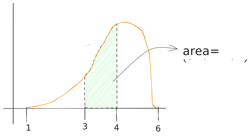
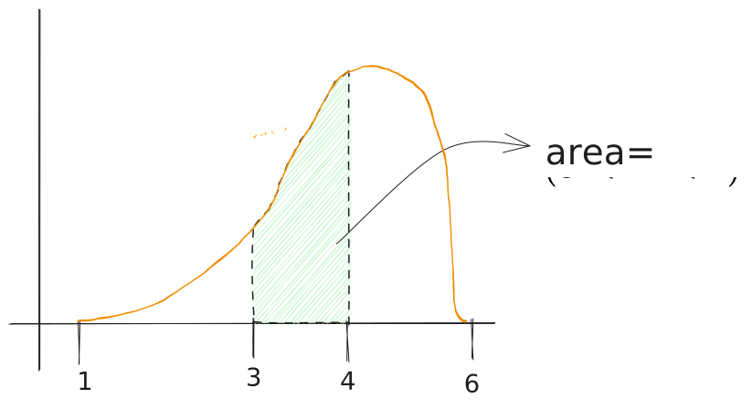
Suppose X∈(1,6), and X’s probability density function looks like this. For the sake of example, let’s say we are looking for P(3<X<4). This value can be found by calculating the area under the graph in that given interval. Applying principles from calculus, we know that the area is equal to ∫34fX(t)dt
The cumulative distribution functionFX (of a continuous random variable X) is defined as:
FX(a)=∫−∞af(t)dt
This is the area under the graph up toa.
By no coincidence, this is also P(X<a)
This function is useful because P(a<X<b)=FX(b)−FX(a).
It saves us from having to repeatedly calculate integrals at every step, by doing it once at the beginning.
Continuing from previous example
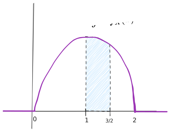
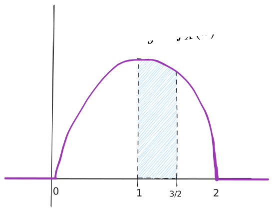
fX(x)={43(2x−x2)00<x<2otherwise FX(x)=⎩⎨⎧0∫0x43(2t−t2)dt1x<00<x<2x>2
That’s very nice and all, but we want to avoid repetitive integration, so we calculate it here:
∫0x43(2t−t2)dt=43(x2−3x3)
Our final cumulative distribution function looks like this:
FX(x)=⎩⎨⎧043(x2−3x3)1x<00<x<2x>2
So if we want to find P(1<X<32), all we need to do is FX(32)−FX(1)