ODEs· Note 03
Autonomous Equations
Slope Field
Definition: Slope Field
A slope field is a tool we can use to learn information about the solutions to an ODE even when we cannot solve it completely.
Using ODE, we look at many points in the plane and calculate the slope of a tangent to any solution at that point. By doing this for many points, we can see what graphs of solutions look like.
Autonomous Equations
An ODE is autonomous if it is in the form .
For example,
What does the slope field of an autonomous equation look like?
Since depends only on y, the slope of any solution is constant along any horizontal line.
Given the ODE , we can find the slopes for any given y:
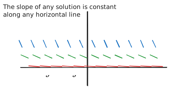
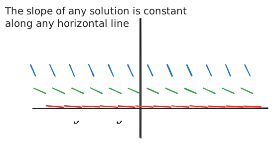
An autonomous ODE is a type of separable ODE, so we have an equilibrium solution for any satisfying .
In our example, , so is an equilibrium solution to this ODE.
Actual Solutions to the ODE
For the ODE :
The equilibrium solution is .
To solve:
Here, the uniformity of the slope along each horizontal line is very clear, because each solution is a right/left translation of the graph .
y = \frac{1}{x + C_1}
y = \frac{1}{x + C_2}
y = \frac{1}{x + C_3}
C_1=-1
C_2=0
C_3=1
Sketching Solutions of an Autonomous ODE
We’ll be using the equation .
- Sketch the equilibrium solutions for each root of
-
- Sketch (on a separate pair of axes) the graph of as a function of , or at least investigate where is positive/negative, increasing/decreasing, and find the extreme points.
- Sketch the function as
- Find the roots (we already did this in step one)
- 1, 0
- Examine the expanded form
- Identify the extreme points
- 2nd derivative is
- Root of 2nd derivative is
- Graph is a “frowning” parabola, so our extreme point is a maximum
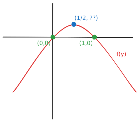
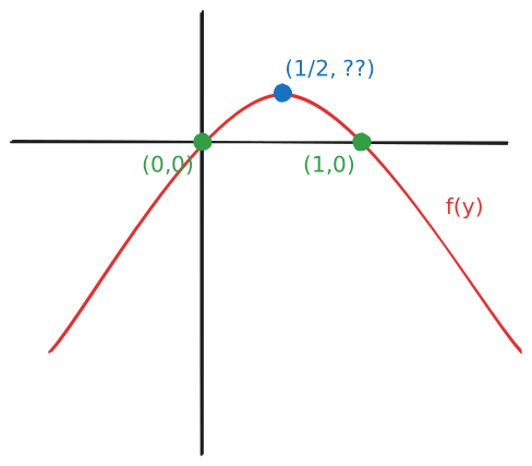
- Examine the “signs” of :
- For arguments where is decreasing
- For arguments where is increasing
- For arguments where we already know this is an equilibrium solution
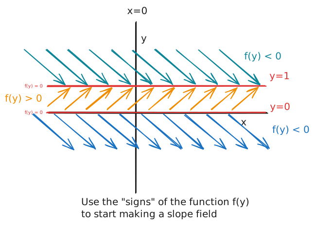
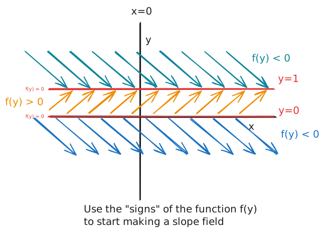
- Find the concavity of the solutions
- In an autonomous ODE,
-
- is concave up
- i.e. is positive and increasing
- i.e. is negative and decreasing
- is concave up
-
- is concave down
- i.e. is negative and increasing
- i.e. is positive and decreasing
- is concave down
- and changing sign is an extreme point of
- y(x) has an inflection point
- In our example, only changes signs at it’s single root (see step 2.4.2), so that is our single point of inflection.
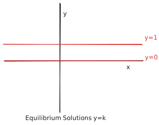
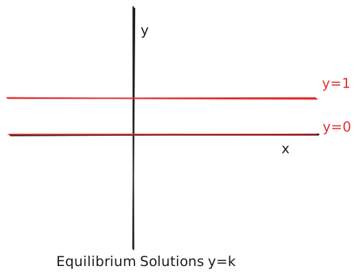
Given the above calculations and sketches, we examine the behavior of f, f’, y’’ as y passes through the values , since those were our equilibrium solutions and inflection points:
| is… | ||||
|---|---|---|---|---|
| Concave down | ||||
| Concave up | ||||
| Concave down | ||||
| Concave up |
We can now sketch the slope field of the solutions:
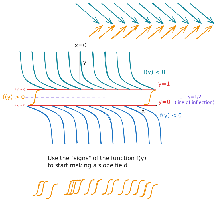
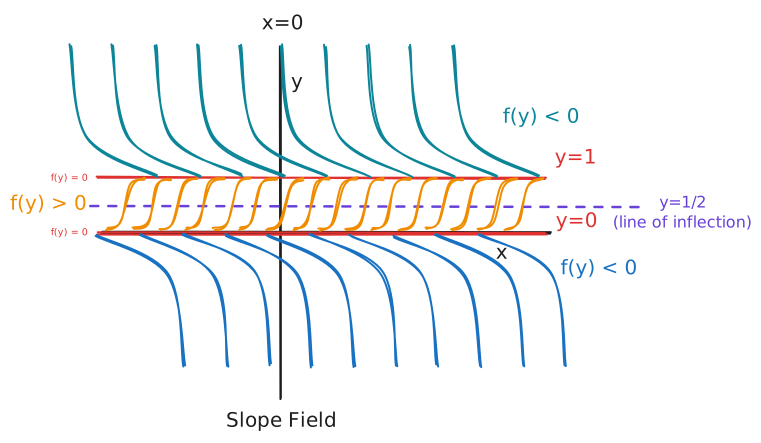
Summary
- Find the equilibrium solutions: where
- Find where is positive/negative/increasing/decreasing, and find the extreme points.
- If then is increasing along the line
If then is decreasing along the line
- If have the same sign () at , then is concave up along the line
- If have different signs () at , then is concave down along the line
- If at , has an inflection point along the line . This line is called a line of inflection.
Classification of Autonomous ODE Solutions
The equilibrium solutions of an AODE can be classified as one of three types:
- Stable:
- If strays slightly from the equilibrium, then it will move towards it as increases
- Unstable:
- If strays slightly from the equilibrium, then it will move further away it as increases
- Semi-Stable:
- Stable in one direction of (up or down), and unstable in the other direction.