Calculus I· Note 04
Graph Sketching
May 22 Lecture. Links to the board and the recording.
Definition:
is an extreme point of if there exists a neighborhood of , such that either or
In the first case, is a local maximum; in the second case, is a local minimum.
Fermat’s Theorem (#36)
If is differentiable at , and is an extreme point of , then
Caveats:
- Note the condition is differentiable at :
- can have an extreme point where f is not differentiable.
Ex.:
- Not every point where is an extreme point. (i.e., the converse of Fermat’s theorem is not true.)
Critical points
By Fermat’s Theorem, the only candidates for extreme points of are points where
- is not differentiable at
If satisfies either of these conditions, then is a critical point of .
Rolle’s Theorem
Suppose is continuous in and differentiable in , with . Then
Mean Value Theorem (MVT)
Suppose is continuous in and differentiable in . Then,
Practically speaking, there exists at least one point on between where the slope of the tangent is exactly equal to the slope of the line between and .
You can think of this as a “sideways” version of Rolle’s Theorem.
Corollaries of MVT:
- If for all , then is constant.
- Let be continuous on , and differentiable on . If , then they differ by a constant (i.e. for some constant k on all of )
- If is differentiable on and then f is increasing on .
- If is differentiable on and then f is decreasing on .
- is increasing
- is decreasing
- Linear Approximation:
For h small,
See: Explanation
Sketching graph using information about
Ex.:
We wish to find extreme points where is increasing and where is decreasing.
- Find critical points (where or is not differentiable)
- is a polynomial, so it’s differentiable for all
- (set it to be zero to find extreme points)
- Critical points are
- Examine critical points
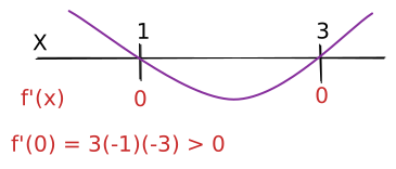
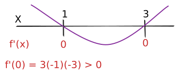
- First derivative test:
- For local maximum,
For local minimum, - Check the signs of the derivative function using the snake method
- is a local max
is a local min
- For local maximum,
- method to locate extreme points (from the critical points):
- Look at the second derivative where is a critical point
- If then is a local min
- If then is a local max
- If then this test gives no information
- In our example, , so we check:
- , so it’s a local maximum
- , so it’s a local minimum
- First derivative test:
- Sketch the graph
- Plot the points where the graph intersect the X-axis
- Plot the maxima and minima
- connect them using information gleaned from examination of critical points.
May 22 Tirgul. Links to the board and recording.
[Incomplete]
[Incomplete until End of Unit Lecture June 5]